In [1]:
%load_ext rpy2.ipython
- R code can be mixed with Python code
- Cells with R code are prefixed with
%%R - The R output is returned
In [2]:
%%R

R.version
In [3]:
%%R
## Dobson (1990) Page 93: Randomized Controlled Trial :
counts <- c(18,17,15,20,10,20,25,13,12)
outcome <- gl(3,1,9)
treatment <- gl(3,3)
print(d.AD <- data.frame(treatment, outcome, counts))
glm.D93 <- glm(counts ~ outcome + treatment, family = poisson())
anova(glm.D93)
Communicating with the outside world (Python)
In [4]:
FILENAME = "Pothole_Repair_Requests.csv"
| "`-i`": | into R |
| "`-o`": | out of R |
In [5]:
%%R -i FILENAME -o result
print(FILENAME)
result <- 2*pi
In [6]:
print(result)
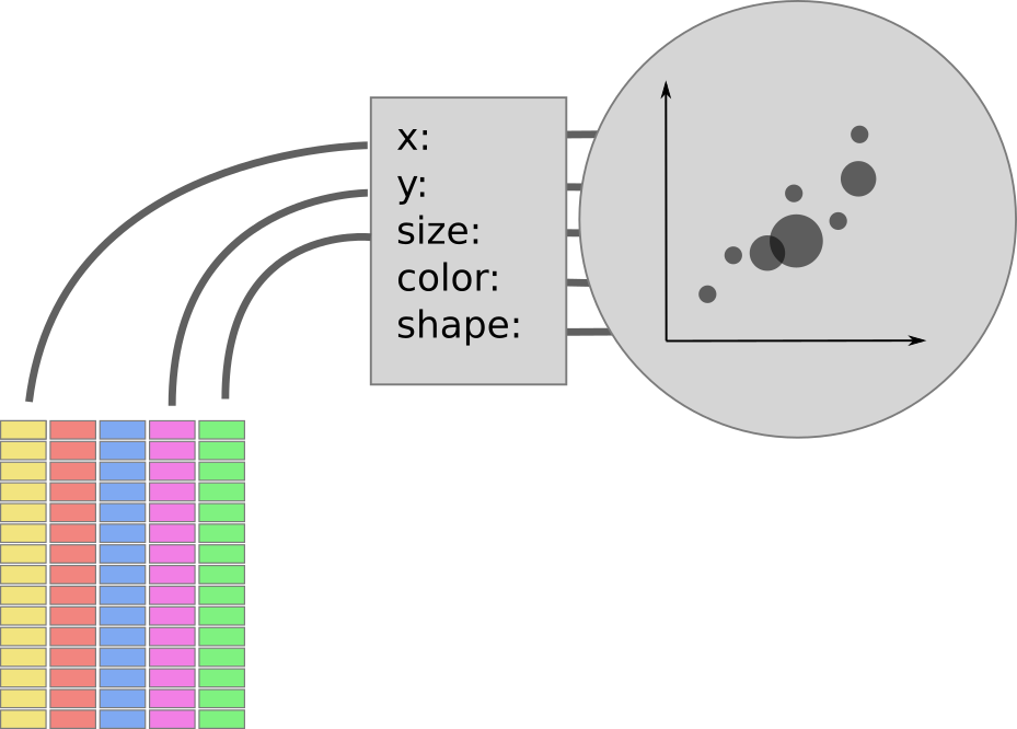
Data table
- Running code in 2 languages is nice...
- ...but code objects should be passed back and forth
- The "data table" is:
- a high-level data structure
- common (in concept) across Python, R (and SQL, etc...)
Dataset
|

|


| mutate | modify/add column |
| filter | filter rows |
| select | select columns |
| group_by | group rows |
| summarize | summarize groups of rows |
In [27]:
from rpy2.robjects.lib import dplyr
ddataf = dplyr.DataFrame(dataf)
Strings as R code
In [28]:
ddataf = \
    (ddataf.
     mutate(date_submit='as.POSIXct(Date.Submitted, ' + \
	                '           format="%m/%d/%Y %H:%M:%S")',
            date_complete='as.POSIXct(Date.Completed, ' + \
	                '           format="%m/%d/%Y %H:%M:%S")').
     mutate(days_to_fix='as.numeric(date_complete - date_submit, ' +\
                                    'unit="days")'))
In [29]:
dataf_plot = ddataf.filter('Status == "Closed"')
p = (gp.ggplot(dataf_plot) +
     gp.geom_density(gp.aes_string(x='days_to_fix')) +
     gp.facet_grid('~Status') +
     gp.scale_x_sqrt() +
     gp.theme_gray(base_size=15) +
     gp.theme(**{'legend.position': 'top'}))
p
Out[29]:

In [30]:
p = (gp.ggplot(ddataf.filter('Status == "Closed"',
                             'days_to_fix < 100')) +
     gp.geom_histogram(gp.aes_string(x='days_to_fix'), bins=100) +
     gp.facet_grid('~Status') +
     gp.theme_gray(base_size=15) +
     gp.theme(**{'legend.position': 'top'}))
p
Out[30]:

Extract coordinates from column "Address"
In [31]:
col_i = ddataf.colnames.index('Address')
first_address = next(ddataf[col_i].iter_labels())
first_address
Out[31]:
In [32]:
s_pat_float = '[+-]?[0-9.]+'
s_pat_coords = '.+\((%s), (%s)\)$' % (s_pat_float, s_pat_float)
import re
pat_coords = re.compile(s_pat_coords,
                        flags=re.DOTALL)
pat_coords.match(first_address).groups()
Out[32]:
Final function
In [33]:
from rpy2.robjects import NA_Real
def extract_coords(address):
    m = pat_coords.match(address)
    if m is None:
        return (NA_Real, NA_Real)
    else:
        return tuple(float(x) for x in m.groups())

extract_coords(next(ddataf[col_i].iter_labels()))
Out[33]:
Python and R entwinned
In [34]:
from rpy2.robjects.vectors import FloatVector
from rpy2.robjects import globalenv

globalenv['extract_lat'] = \
    lambda v: FloatVector(tuple(extract_coords(x)[0] for x in v))

globalenv['extract_long'] = \
    lambda v: FloatVector(tuple(extract_coords(x)[1] for x in v))

ddataf = \
    (ddataf.
     mutate(lat='extract_lat(as.character(Address))',
            long='extract_long(as.character(Address))'))
In [35]:
p = (gp.ggplot(ddataf) +
     gp.geom_hex(gp.aes_string(y='lat', x='long'), bins=50) +
     gp.scale_fill_continuous(trans="sqrt") +
     gp.theme_gray(base_size=15) +
     gp.facet_grid('~Status'))
p
Out[35]:

In [36]:
dtf_grp_r = 'cut(days_to_fix, c(0,1,5,30,60,1500))'
p = (gp.ggplot(ddataf.filter('Status == "Closed"')) +
     gp.geom_point(gp.aes_string(y='lat', x='long',
                                 color=dtf_grp_r),
                  size=1) +
     gp.facet_grid('~Status') +
     gp.theme_dark(base_size=15) +
     gp.scale_color_brewer("Days to fix"))
p
Out[36]:

In [37]:
p = (gp.ggplot(ddataf.filter('Status == "Closed"')) +
     gp.geom_histogram(gp.aes_string(x='date_complete'), bins=30) +
     gp.facet_grid('~Status') +
     gp.theme_gray(base_size=15) +
     gp.theme(**{'legend.position': 'top'}))
p
Out[37]:

In [38]:
p = (gp.ggplot(ddataf.filter('Status %in% c("Closed", "Resolved")')) +
     gp.geom_hex(gp.aes_string(x='date_submit', y='date_complete')) +
     gp.facet_grid('~Status') +
     gp.scale_fill_continuous(trans="log") +
     gp.theme(**{'legend.position': 'top',
                 'axis.text.x': gp.element_text(angle=45, hjust=.5)}))
p
Out[38]:

In [39]:
extract_weekday = """
factor(weekdays(date_submit),
       levels=c("Sunday", "Monday",
                "Tuesday", "Wednesday", "Thursday",
                "Friday", "Saturday"))
"""
# transition iPhone / iOS
ddataf = (ddataf.
          mutate(year_submit='format(date_submit, format="%Y")',
                 month_submit='format(date_submit, format="%m")',
                 weeknum_submit='as.numeric(format(date_submit+3, "%U"))',
                 weekday_submit=(extract_weekday)).
                 filter('year_submit >= 2012',
                 'Platform != ""'))
In [40]:
from IPython.core import display
p = (gp.ggplot(ddataf) +
     gp.geom_bar(gp.aes_string(x='(weekday_submit)', fill='Platform')) +
     gp.scale_fill_brewer(palette = 'Set1') +
     gp.scale_y_sqrt() +
     gp.theme(**{'axis.text.x': gp.element_text(angle = 90, hjust = 1)}) +
     gp.facet_grid('month_submit ~ year_submit'))
display.Image(display_png(p, height=700))
Out[40]:

In [41]:
by_weekday = ddataf.group_by('weekday_submit')
n_platforms_weekday = (by_weekday.
                       summarise(n='length(unique(Platform))'))
print(n_platforms_weekday)